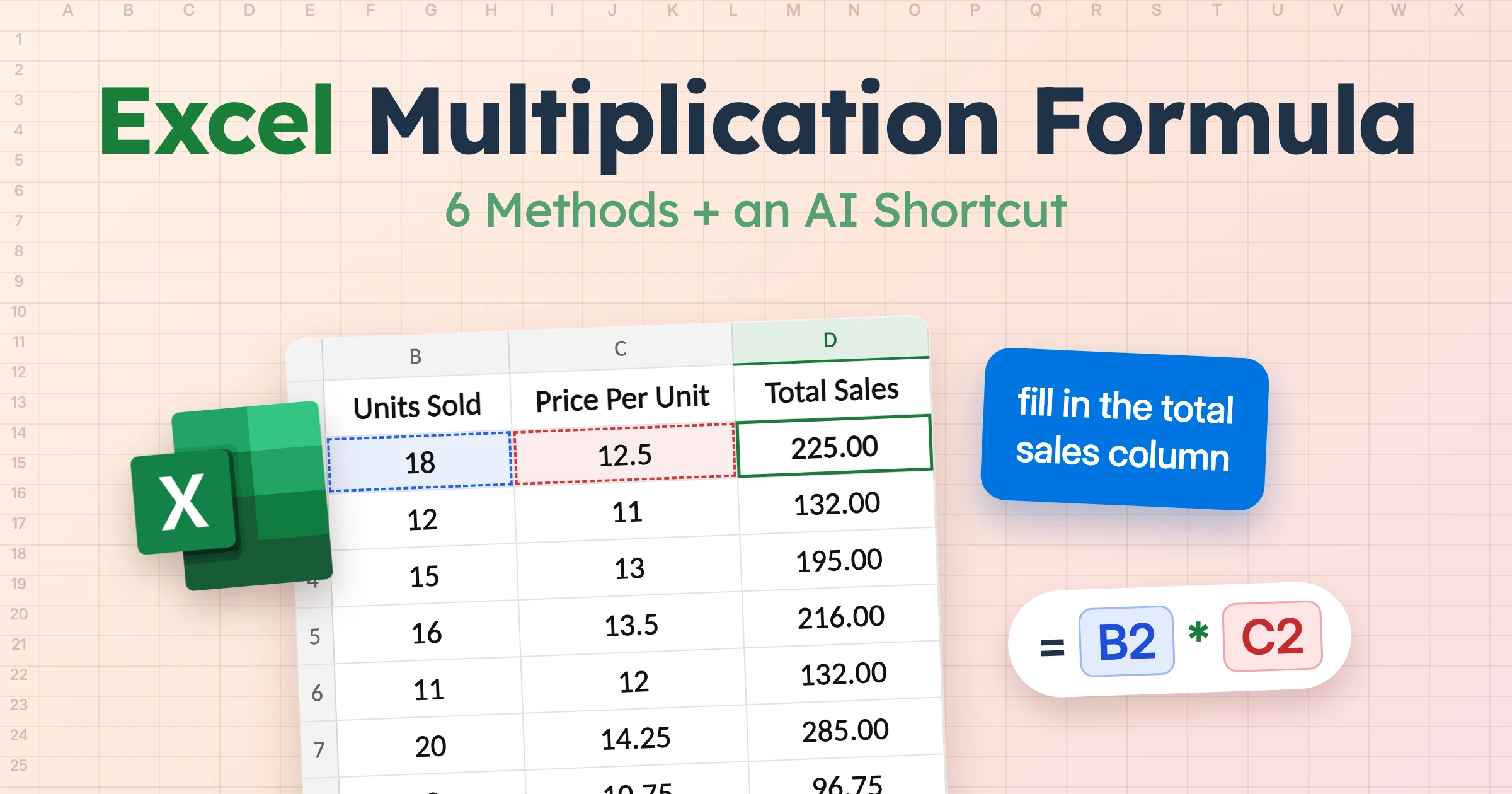
The basic Excel multiplication formula is =B2*C2. Excel uses an asterisk (*) instead of the × symbol, so if B2 holds the units sold and C2 holds the price per unit, the formula multiplies the two values and returns the total.
That same formula works for simple calculations. The setup changes when you need to multiply an entire column, keep one multiplier fixed, multiply several cells at once, or add up the products from multiple rows.
If you copy a formula without fixing a reference that should stay constant, Excel adjusts that reference as the formula moves down the column. That can leave you with zeros or incorrect totals even when the first row looks right.
Below, you'll learn how to multiply in Excel for each of these situations, starting with the simplest method.
Excel Multiplication Formula Basics
Excel does not have a function named MULTIPLY. For basic calculations, a multiplication formula in Excel uses the asterisk (*) operator. When you need to multiply several cells or a range, you can also use the PRODUCT function.
Every formula starts with an equals sign (=), which tells Excel to calculate what follows.
Most multiplication formulas take one of these forms:
=8*5
=B2*C2
=D2*$G$1
The first multiplies two numbers, the second multiplies values from two cells, and the third multiplies a cell by a fixed value. That fixed reference is important when you copy a formula down a column, and you'll see it in more detail below.
Two small typing mistakes can break the formula. If you use x instead of * with cell references, Excel can return a #NAME? error. If you leave out the equals sign, Excel will not treat the entry as a formula.
Both the asterisk and PRODUCT work in every version of Excel, including Excel for Mac and Excel for the web.
Method 1: Multiply Two Cells With the Asterisk
To multiply two cells in Excel, click the cell where you want the result, type =, click the first cell, type *, click the second cell, and press Enter.
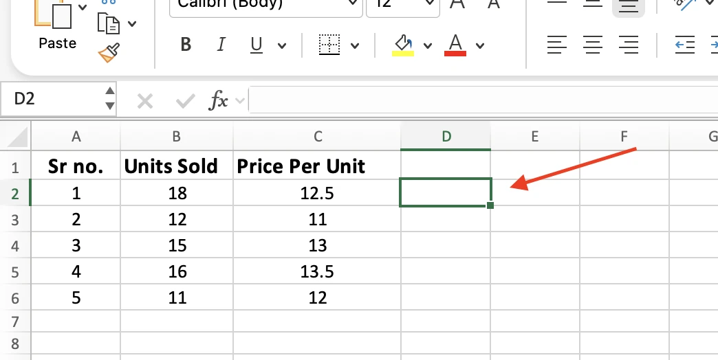
Here is how that works on a simple sales sheet. Column B holds units sold, column C holds the price per unit, and column D is where you want the total.
Step 1: Click the result cell
Click cell D2. This is where your total will appear.
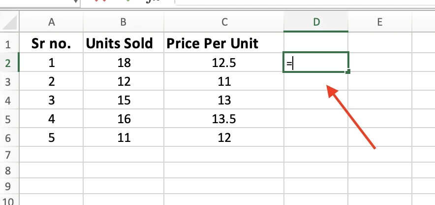
Step 2: Start the formula
Type =. Excel now treats everything you type next as a calculation.
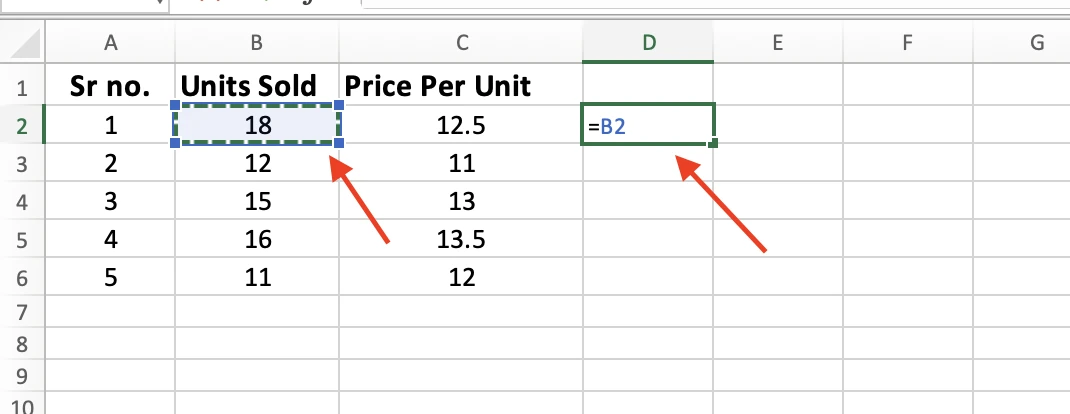
Step 3: Click the first cell
Click cell B2, which contains 18. Excel adds B2 to the formula and outlines that cell in color.
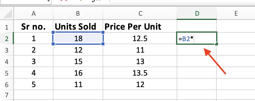
Step 4: Add the asterisk
Type *. This is the multiplication symbol in Excel.
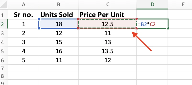
Step 5: Click the second cell
Click cell C2, which contains 12.50. Your formula is now complete.
Step 6: Press Enter
Hit Enter. D2 returns 225, and the formula bar shows =B2*C2.
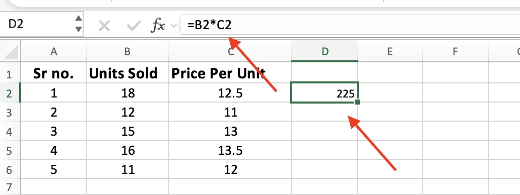
If the cell is formatted as currency, Excel may display the result as $225.00.
Clicking the cells instead of typing their references can help you avoid entering the wrong cell address. If the cells are far apart, though, typing the references directly may be faster.
Method 2: Multiply Two Columns Row by Row
To multiply two columns, write the formula once in the top row, then double-click the fill handle to copy it down the whole column.
A common spreadsheet task is multiplying units sold by price per unit, where every row needs its own total.
Step 1: Write the formula in the first row
In cell D2, enter =B2*C2 and press Enter.
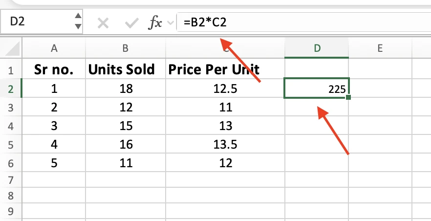
Step 2: Select the formula cell
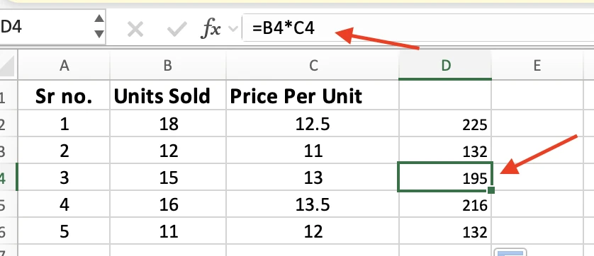
Click D2 once. A small square appears at the bottom-right corner of the cell. That square is the fill handle.
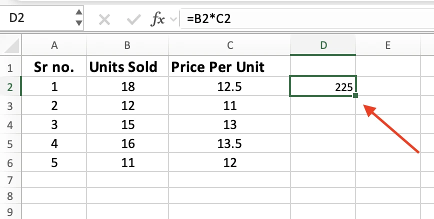
Step 3: Fill the formula down
Hover over the fill handle until your cursor turns into a black cross, then double-click. Excel copies the formula down to the last row of your data.
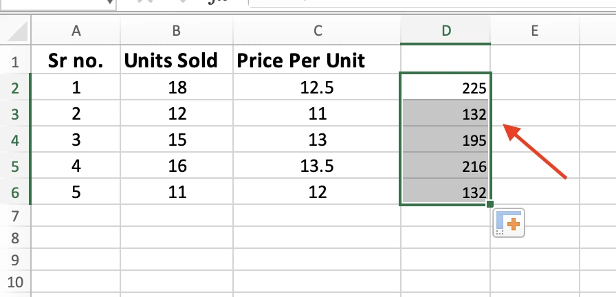
Double-clicking fills only as far as the neighboring column has data, so it stops at the first blank row. If your data has gaps, dragging gives you more control over exactly how far the formula is copied.
Each row now holds its own formula. D3 reads =B3*C3, D4 reads =B4*C4, and so on. Excel shifted both references down one row at a time, which is exactly what you want here.
The One-Formula Alternative
If your version of Excel supports dynamic arrays (Microsoft 365 and Excel 2021 or later), you can return all the row-by-row results from one formula:
=B2:B6*C2:C6
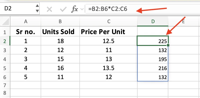
Enter it in D2, and the results spill into the cells below. Only the top cell contains the editable formula, so you do not need to copy it down manually.
If you are using an older version of Excel, use =B2*C2 and fill the formula down instead.
You can multiply rows in Excel the same way when your data runs across instead of down. If row 2 holds the units sold and row 3 the price per unit, enter =B2*B3 in B4, then drag the fill handle to the right instead of down.
Method 3: Multiply an Entire Column by the Same Number
To multiply a whole column by one fixed number, lock that number's cell with dollar signs, then fill the formula down. The formula is =D2*$G$1.
Without the dollar signs, the reference moves as you fill the formula down. The next row points at G2 instead of G1, and Excel treats that empty cell as 0.
Say you want to reduce every total in column D by 10%. Instead of typing the discount into every formula, you can store one multiplier in a separate cell and use it for every row.
Step 1: Put the number in its own cell
Type 0.9 into cell G1. This is the multiplier for a 10% discount. Label F1 as Discount Multiplier so you know what the value represents.
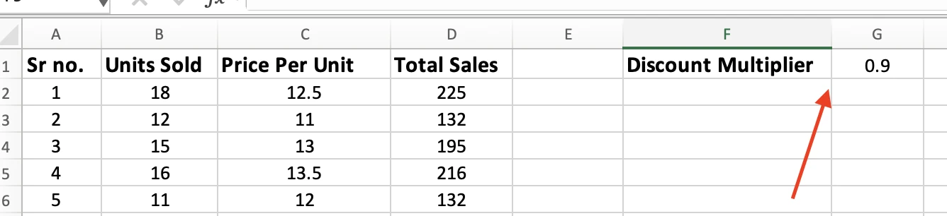
Keeping the number in a cell means you change it once and every row updates.
Step 2: Write the formula with dollar signs
In cell E2, enter:
=D2*$G$1
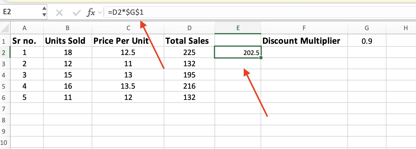
D2 contains the first total, 225, and G1 contains 0.9, so Excel returns 202.5 in E2.
$G locks the column and $1 locks the row, so the formula keeps pointing at G1 no matter which row it lands in.
Step 3: Fill it down
Double-click the fill handle. Click any cell in column E and the formula bar still shows $G$1.
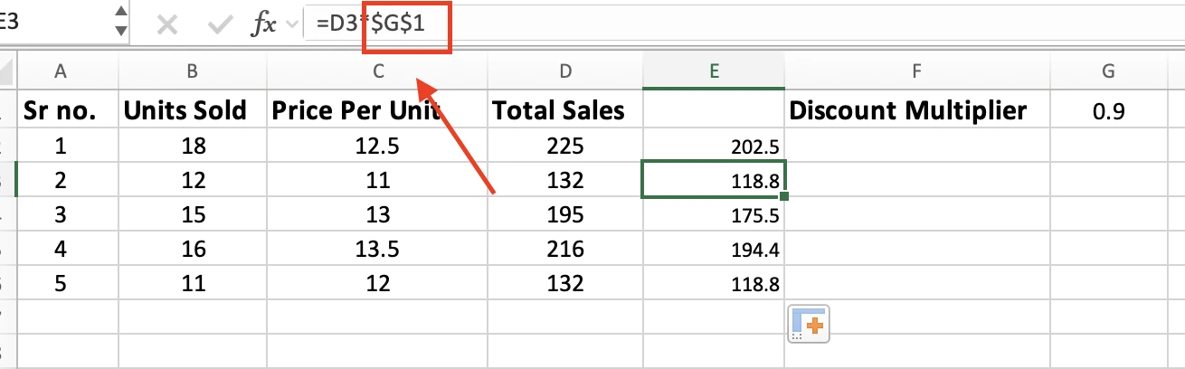
Change G1 from 0.9 to 0.8 and all five discounted totals update at once.
The Shortcut for Adding Dollar Signs
You do not have to type the dollar signs manually. Select the cell reference in the formula bar and press F4 to cycle through the four reference types:
Press F4 | Reference | What stays fixed |
|---|---|---|
Once | $G$1 | Column and row |
Twice | G$1 | Row only |
Three times | $G1 | Column only |
Four times | G1 | Nothing |
On a Mac, press Command + T to switch between the same reference types. F4 works too, but most Mac keyboards need Fn held with it.
For this multiplication method, you want both the column and row fixed because every formula should keep pointing to G1. If the reference should change as you copy the formula, leave it as G1.
Method 4: Multiply Multiple Cells With the PRODUCT Function
Excel's multiplication function is PRODUCT.
=PRODUCT(B2,C2) returns 225, the same as =B2*C2.
PRODUCT becomes more useful when you need to multiply a longer range. Instead of chaining many cell references together with asterisks, you can reference the whole range in one formula.
Step 1: Start the function
Click the cell where you want the answer and type =PRODUCT(. A tooltip appears showing what the function expects.
![Typing =PRODUCT( in D2 with the tooltip PRODUCT(number1, [number2], ...) shown below](/_next/image?url=%2Fimages%2Fblog%2Fexcel-multiplication-formula-product-tooltip.webp&w=3840&q=75)
Step 2: Select the cells to multiply
Click B2, type a comma, then click C2.
=PRODUCT(B2,C2)
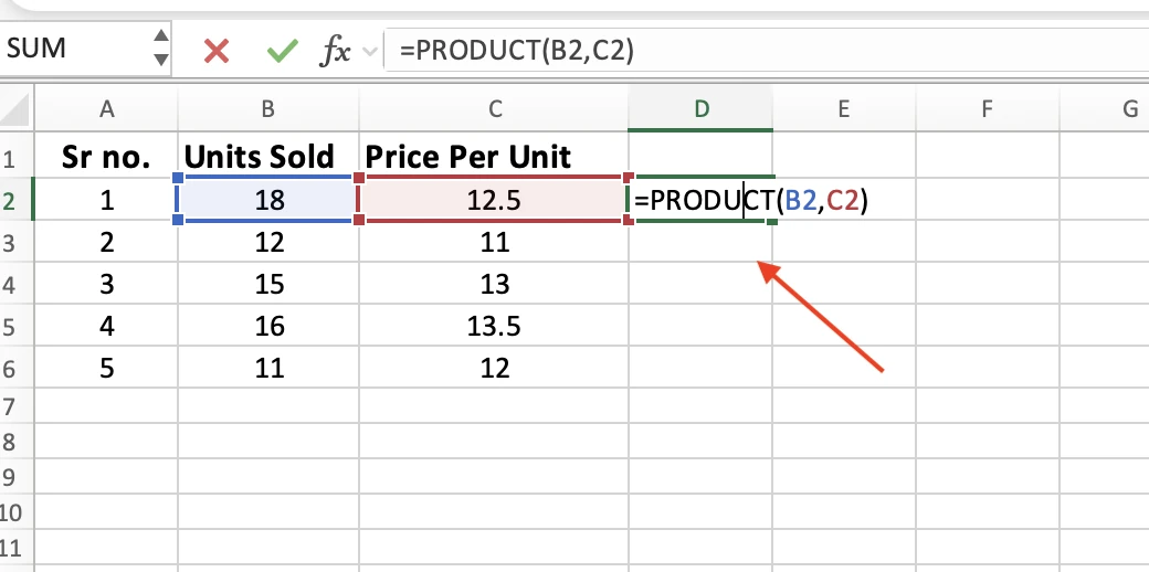
If the cells are scattered around the sheet, separate each cell reference with a comma. To multiply a whole run of cells, drag across them instead and Excel writes the range for you.
Step 3: Close the parenthesis and press Enter
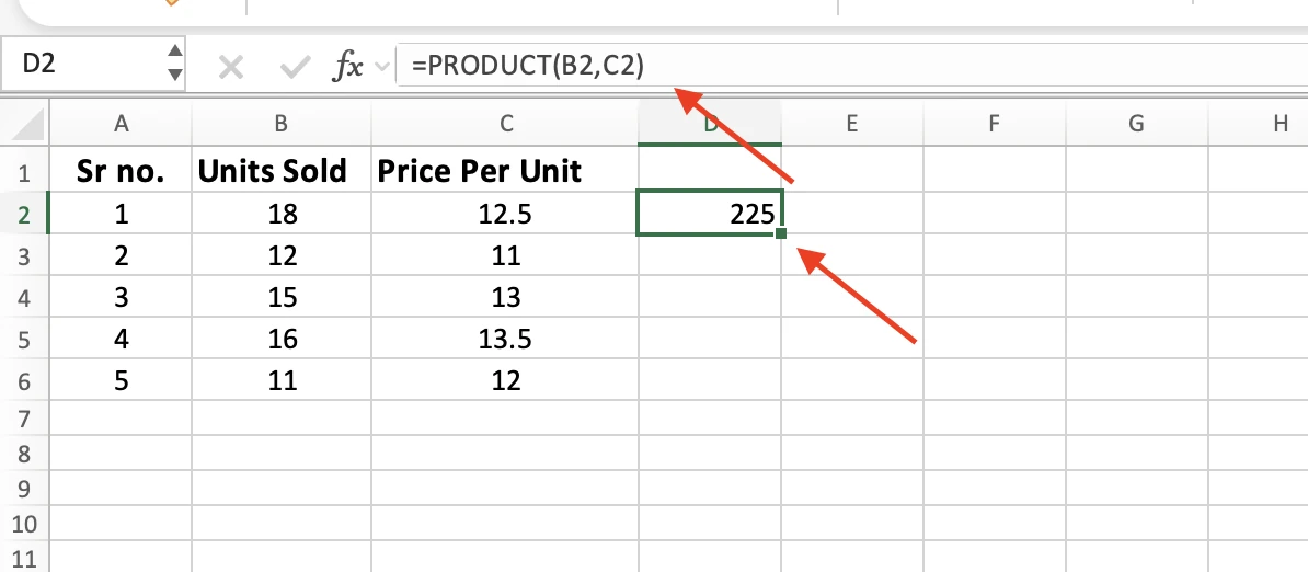
Type ) and hit Enter. The cell returns 225.
When to Use PRODUCT Instead of the Asterisk
Use PRODUCT when you multiply more than two or three values. Say a row holds five factors in H2:L2: units sold, price per unit, a discount, a tax rate and an exchange rate. The asterisk version is long:
=H2*I2*J2*K2*L2
With PRODUCT, you can write the same calculation as:
=PRODUCT(H2:L2)
PRODUCT also handles text differently. It skips any text in a referenced range, including numbers stored as text, so the result can be quietly wrong. The asterisk tries to convert text to a number and returns #VALUE! only when it can't, for example with a word like "N/A". Blank cells differ too: =B2*C2 returns 0 when C2 is empty, while =PRODUCT(B2,C2) skips the blank and returns 18.
You can also mix ranges and numbers in the same formula:
=PRODUCT(B2:C2,0.9)
This multiplies units sold by price per unit, then by 0.9, the discount multiplier from Method 3. For row 2, it returns 202.5.
Method 5: Multiply by a Percentage in Excel
To multiply by a percentage, include the percent sign in the formula. =D2*20% gives you 20% of the value in D2, because Excel reads 20% as 0.2.
Suppose you need 20% of every total, because that is the commission on each sale.
Step 1: Click the result cell
Click cell E2, next to the first total.
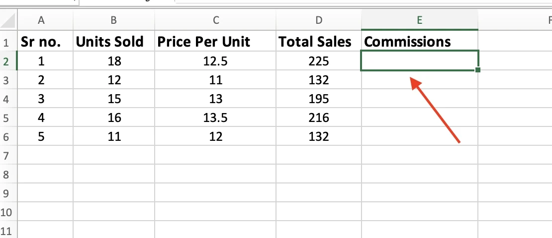
Step 2: Write the formula
Enter the formula with the percent sign included:
=D2*20%
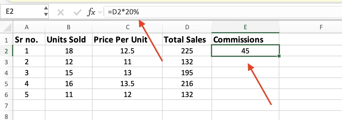
Leave the percent sign out and the formula still runs, but it gives you the wrong result. =D2*20 multiplies by twenty, returning 4,500 instead of 45, and Excel shows no error because multiplying by 20 is a valid thing to do.
Step 3: Press Enter and fill down
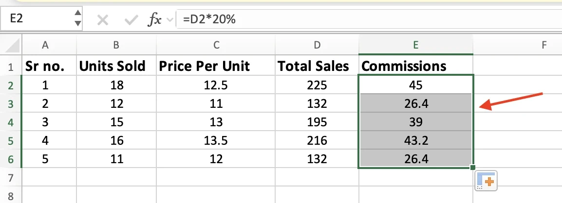
E2 returns 45. Double-click the fill handle and every row gets its own commission figure.
Increase or Decrease by a Percentage
To increase a value by a percentage, add the percentage to 1 inside parentheses:
=D2*(1+20%)
That returns 270. To reduce the value by 20%, subtract instead:
=D2*(1-20%)
That returns 180.
Using a Percentage From Another Cell
Typing 20% into every formula means editing every formula when the rate changes. Put the rate in its own cell, such as H1, and lock it the same way you did in Method 3:
=D2*$H$1
With 20% in H1, E2 returns 45 again, and changing H1 updates every row. For an increase or a decrease, use =D2*(1+$H$1) or =D2*(1-$H$1).
Method 6: Multiply and Add With SUMPRODUCT
SUMPRODUCT multiplies two columns row by row and adds all the results into one number. =SUMPRODUCT(B2:B6,C2:C6) returns 900, the total value of every sale on the sheet.
Method 2 gives you a result for every row. This gives you one figure, with no extra helper column.
Step 1: Click the cell for your total
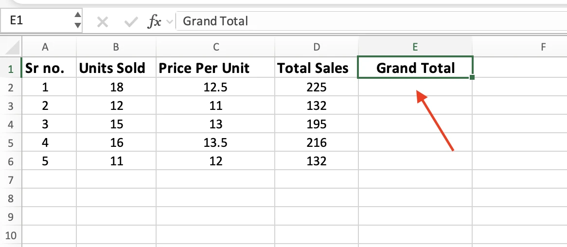
Type "Grand Total" in E1, then click E2. That is where the combined total will appear.
Step 2: Enter the two ranges
Type =SUMPRODUCT(, drag across B2:B6, type a comma, then drag across C2:C6.
=SUMPRODUCT(B2:B6,C2:C6)
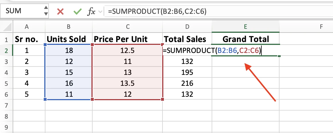
Both ranges must be the same size. If one range has five cells and the other has four, Excel returns #VALUE!.
SUMPRODUCT also treats text as zero, so if any units or prices are stored as text, the total will be too low with no warning.
Step 3: Close the parenthesis and press Enter
Type ) and press Enter. E2 returns 900.
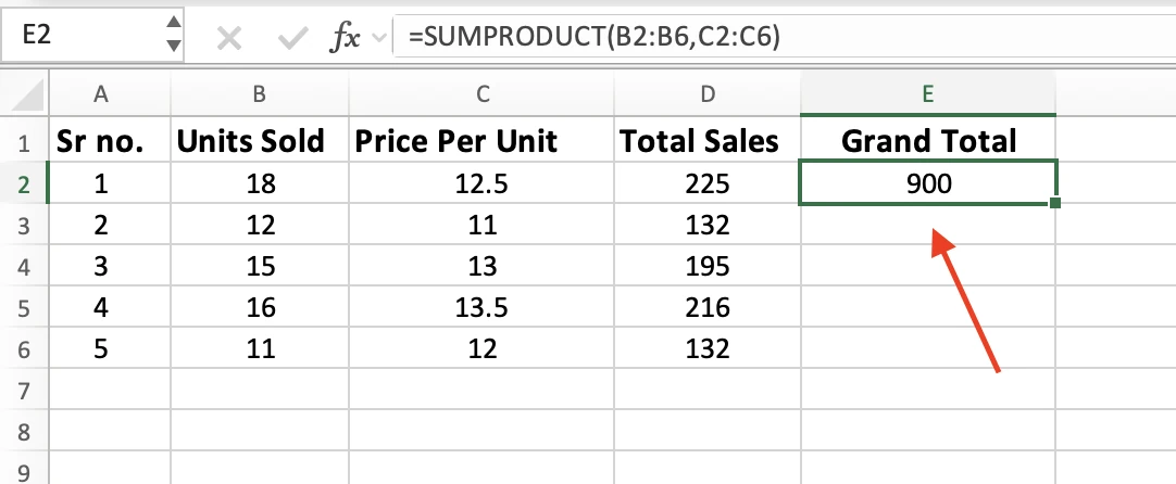
Behind the scenes, Excel multiplies 18 by 12.5, then 12 by 11, and carries on down both columns before adding the five results together.
When to Use SUMPRODUCT Instead of a Helper Column
Use it when the total is the only thing you need. Keep the helper column when you want each row's total too, because SUMPRODUCT returns only the combined total.
If you build column D the way Method 2 does, =SUM(D2:D6) gives you the same 900.
Bonus Method: Let GPT for Excel Clean and Multiply for You
Six methods work, but each one still asks you to know which formula fits the job before you start. That gets harder when the sheet is large or the numbers are not stored cleanly.
GPT for Excel by GPT for Work is an AI agent that works inside your Excel sidebar. You describe the task in plain English, and it can apply the changes directly to your sheet.
Say you have 500 orders where units are typed as "12 units", "16pcs" or "Qty 14", prices mix "13.00 USD" with "US$ 8.99", and a few cells just say "N/A" or "-". A normal multiplication formula returns #VALUE! on all of those rows until you clean them.
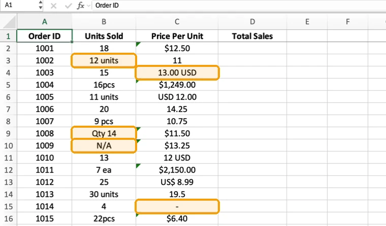
With GPT for Excel, you do not need to describe any of that or know which formula to use. You ask for the result:
"fill in the total sales column"
The agent spotted the messy values on its own and handled the data cleaning first. It cleaned all 500 rows into two new columns, Units (Clean) and Price (Clean), then filled Total Sales with a formula that multiplies them and leaves the 12 orders with a missing value blank. You never write a VALUE, SUBSTITUTE, or TRIM formula.
You can use the same sidebar for much more than formulas. For example, you could enrich 2,000 company names with their website and industry, rewrite 500 product titles to fit a 60-character limit, or tag 10,000 support tickets by urgency and department, each from a single prompt instead of doing the work manually, row by row. You can also compare GPT for Excel with other Excel AI tools if you want a broader look at the options.
You can install GPT for Excel from the Microsoft Marketplace and start with free credits, the usage allowance GPT for Excel draws on as the AI works. No card is needed to try it.
Choosing the Right Multiplication Method
You now have six ways to multiply in Excel, plus GPT for Excel if you want to skip building the formulas yourself. Here is the short version.
If you need to... | Use |
|---|---|
Multiply two cells | =B2*C2 |
Multiply two columns row by row | =B2*C2 filled down |
Use the same multiplier on every row | =D2*$G$1 |
Multiply three or more values | =PRODUCT(H2:L2) |
Calculate or adjust by a percentage | =D2*20%, =D2*(1+20%), or =D2*(1-20%) |
Multiply two columns and get one total | =SUMPRODUCT(B2:B6,C2:C6) |
Skip building formulas manually | GPT for Excel |
The asterisk covers most everyday multiplication, so start there. Use an absolute reference when one value needs to stay fixed as you copy the formula. If you forget it, every row after the first points at the wrong cell.
Test your formula on a few rows first and check the results before filling the rest of the column.
If you'd rather skip the cleanup and formula setup, try GPT for Excel and describe the result you want in plain English.
FAQs
Is there a MULTIPLY function in Excel?
No. Excel uses the asterisk (*) for multiplication. The closest built-in function is PRODUCT, which multiplies numbers or ranges together. For example, =PRODUCT(B2,C2) returns the same result as =B2*C2.
Google Sheets does have a MULTIPLY function, which is why many people look for one in Excel.
Why does my Excel multiplication formula return #VALUE!?
One of the referenced cells contains text that Excel can't read as a number, such as a word, a dash, or a unit like "12 pcs". Numbers stored as text are not the cause, because the asterisk converts them. A non-breaking space copied from a web page also triggers the error, and TRIM does not remove it. Strip it with Find and Replace or with =SUBSTITUTE(B2,CHAR(160),"").
Why does my multiplication formula return 0 when I fill it down?
A reference that should stay fixed may have moved. If you enter =D2*G1 and fill it down, the next row becomes =D3*G2. If G2 is empty, the result can be 0.
Lock the fixed reference instead:
=D2*$G$1
What is the difference between PRODUCT and SUMPRODUCT?
PRODUCT multiplies all the values you give it together and returns one result. SUMPRODUCT multiplies corresponding values from two or more ranges, then adds those products together.
Use PRODUCT for one chain of values and SUMPRODUCT when you want one combined total from matching rows.
Can I multiply cells without writing a formula?
Yes. Enter the multiplier in a spare cell, copy it, select the range you want to change, open Paste Special (Ctrl + Alt + V on Windows, Ctrl + Command + V on Mac), choose Multiply, and click OK.
Paste Special applies the multiplication directly to the selected cells, so keep a copy of the original data if you may need it later.