INDEX MATCH in Excel: How to Use It (With Real Examples)

Picture a sales sheet with a few thousand rows. Your manager wants one number: how much a single product made last quarter.

You could scroll through the sheet and copy it by hand, but one wrong row and the number is off.

This is exactly what INDEX MATCH is for. You give it a product name, and it pulls the matching sales figure directly from the table, from any column. It can even look to the left, which VLOOKUP can't do, and it doesn't break when someone inserts or moves a column.

It's actually two functions working together. MATCH finds which row your product is in. INDEX returns the value from that row. Once you understand this pair, you can look up almost anything in a worksheet, in any direction, across tables of any size.

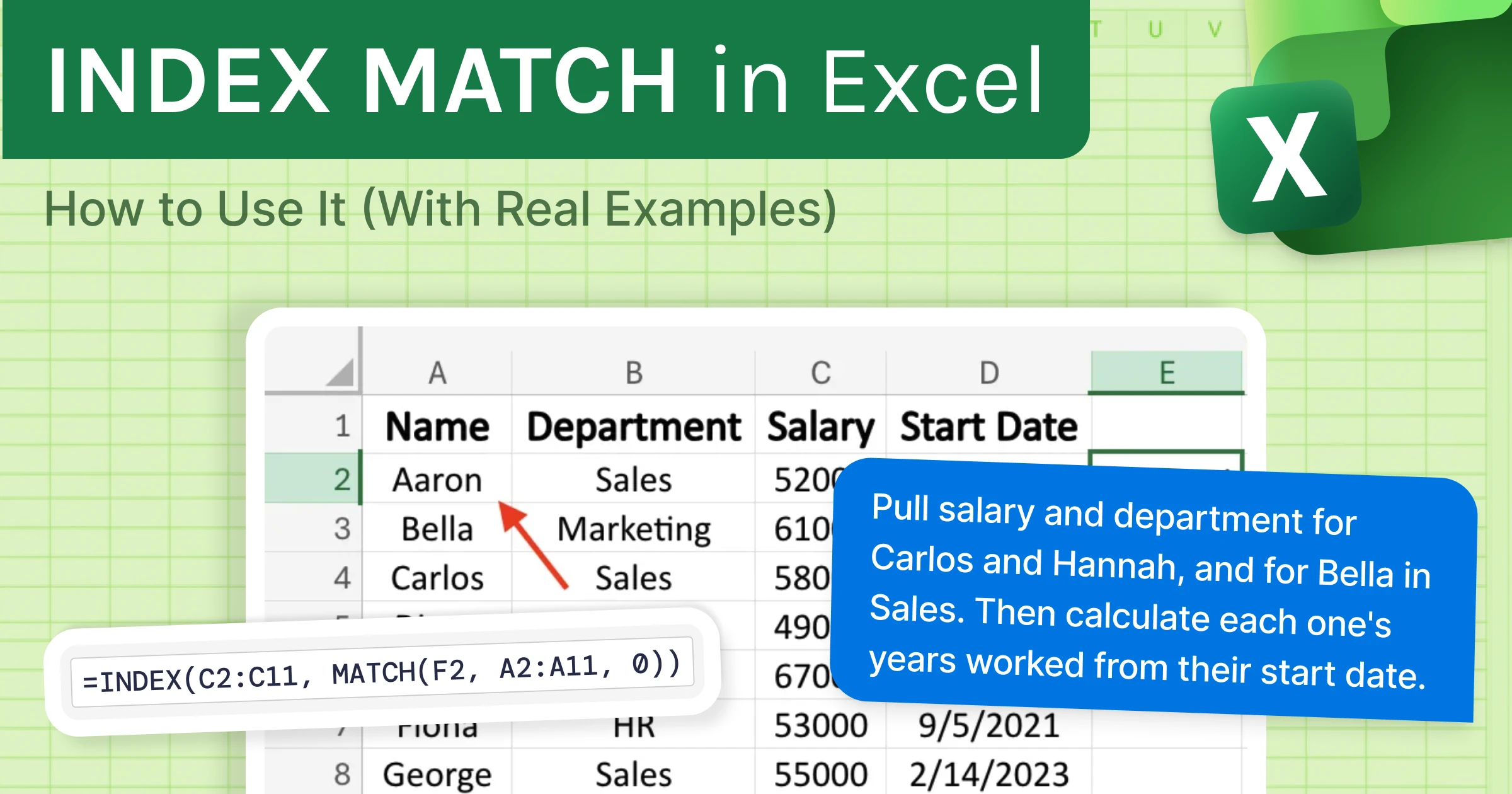
Note: Throughout this guide, we'll use a simple employee table: names in column A, departments in column B, salaries in column C, and start dates in column D, from rows 2 through 11. Paste it into Excel so you can follow along with every example.

What INDEX MATCH Is and How It Works

Start with the two functions on their own. Each does one simple job.

The MATCH function answers a position question: Where is this item in the list?

Suppose you have employee names in column A.

=MATCH("Aaron", A2:A11, 0)

The formula searches the list and tells you that Aaron is the 1st name. Not his salary or department, just his position.

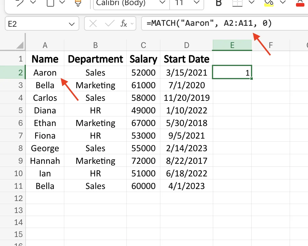
The MATCH function returning the position of the name Aaron in a list of employees

The full syntax is:

=MATCH(lookup_value, lookup_array, match_type)

lookup_value is what you're searching for.
lookup_array is where you're searching.
match_type should almost always be 0, which tells Excel to find an exact match.

The INDEX function does the opposite. You give it a position, and it returns the value at that position.

Since you just learned that Aaron is in position 1, try:

=INDEX(A2:A11, 1)

This returns "Aaron" because it retrieves the value in the first position of the selected range.

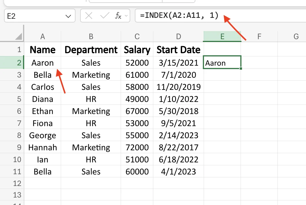
The INDEX function returning the value found at position 1 in a range

The full syntax is:

=INDEX(array, row_num)

array is the range that contains the value you want to return.
row_num is the position within that range.

Here's the key difference between the two functions:

MATCH takes a value and returns its position.
INDEX takes a position and returns the value at that position.

They're essentially mirror images of each other.

That's also why they work so well together. Point INDEX at the salary column instead of the names column, then give it the same position:

=INDEX(C2:C11, 1)

This returns 52000, Aaron's salary. Same row, different column.

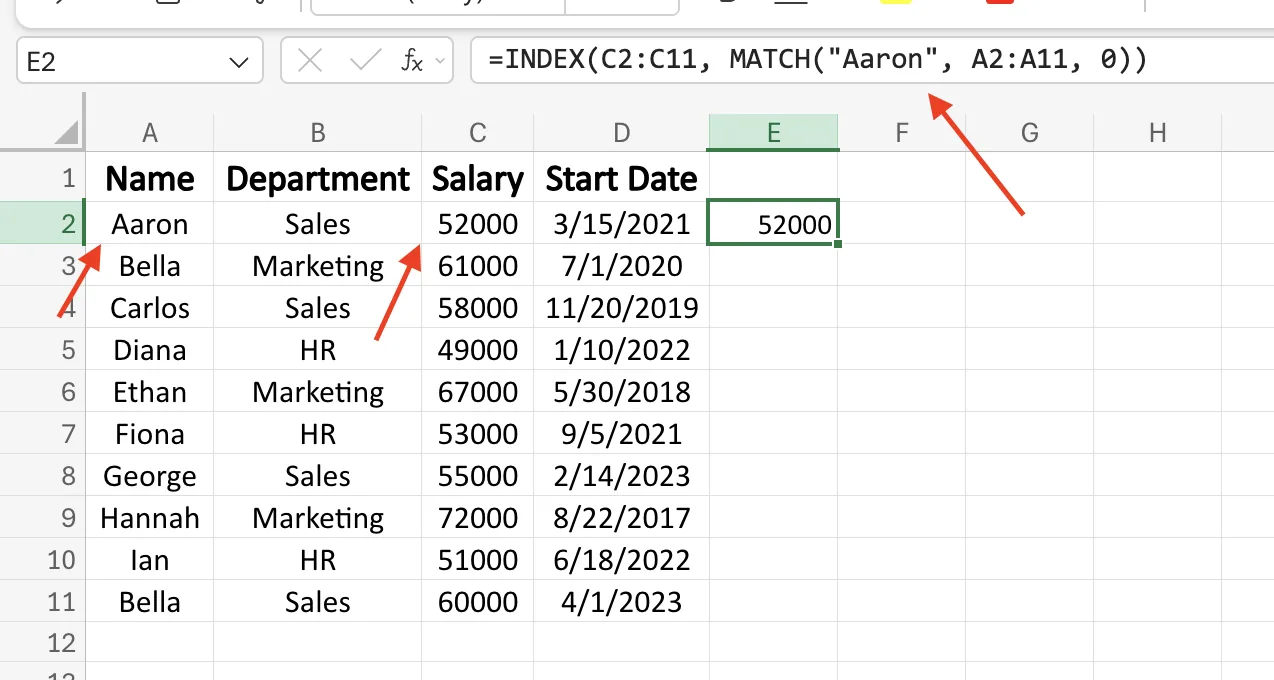
Instead of typing the row number yourself, though, you can have MATCH find it for you:

=INDEX(C2:C11, MATCH("Aaron", A2:A11, 0))

MATCH finds Aaron's position in the names list. INDEX uses that position to return the salary from the salary column.

That's the entire idea behind INDEX MATCH: one function finds the position, and the other returns the corresponding value.

INDEX and MATCH combined to return Aaron's salary from the employee table

How to Use INDEX MATCH in Excel (Basic Example)

On a short list, you can find a salary by eye. On a real worksheet with thousands of rows, that quickly becomes impractical.

So let's build something useful: a simple lookup where you type a name and Excel returns that person's salary.

Pick an empty cell, say F2, and type a name into it, such as Hannah. In the cell next to it, G2, enter:

=INDEX(C2:C11, MATCH(F2, A2:A11, 0))

The formula returns 72000, Hannah's salary. MATCH looks for the name in F2 and finds its position in the names list. INDEX then uses that position to return the matching salary from column C.

Now comes the useful part. Change F2 to Carlos, and G2 instantly shows 58000. Type Diana, and you get 49000. One index match formula answers for anyone on the list. You never touch the formula again, you just change the name.

That's why so many Excel users rely on INDEX MATCH. On a list of 11 names, it saves a few seconds. On a list of 11,000, it saves you from scrolling altogether.

Two-Way Lookup With INDEX MATCH

Sometimes finding the right row isn't enough. You also need the right column. Looking up a student's score in a specific subject is a good example, you have to match both the student and the subject. That's called a two-way lookup.

We'll use a different worksheet for this example because it works with a grid rather than a simple list.

Imagine a table with student names down the left, subjects across the top, and each cell containing a student's score for that subject.

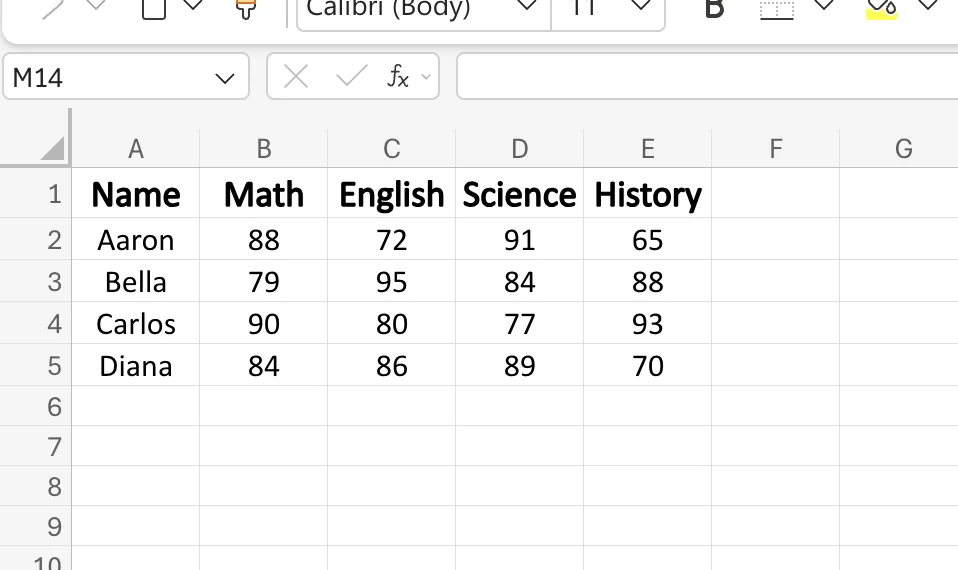
A grid of student scores with names down the left side and subjects across the top

Suppose you want Aaron's Science score. A basic INDEX MATCH formula isn't enough because it only identifies the correct row. To locate a single cell in the grid, you need two MATCH functions: one for the row and one for the column.

First, MATCH finds Aaron's row:

=MATCH("Aaron", A2:A5, 0) returns 1. Aaron is the first student.

Then MATCH finds the Science column:

=MATCH("Science", B1:E1, 0) returns 3. Science is the third subject across.

Now feed both into INDEX. Until now you've given INDEX one position. This time you give it two, a row and a column:

=INDEX(B2:E5, MATCH("Aaron", A2:A5, 0), MATCH("Science", B1:E1, 0))

It returns 91, Aaron's Science score. The first MATCH picked the row, the second picked the column, and INDEX returned the value where they cross.

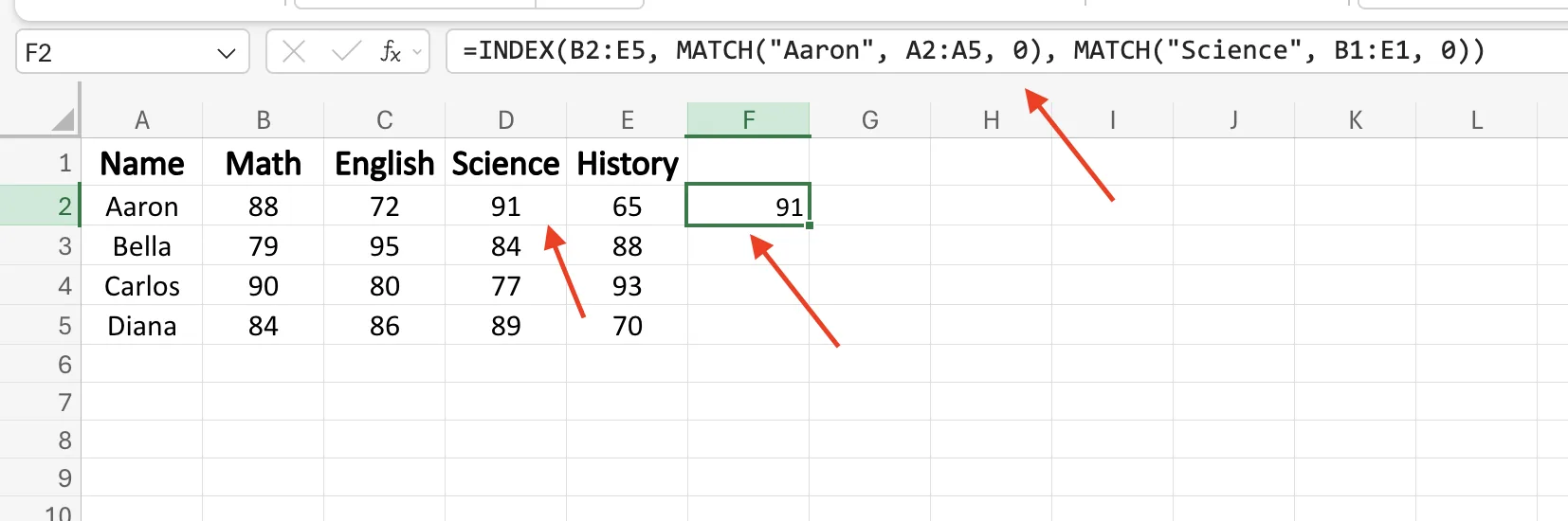
An INDEX MATCH MATCH formula returning Aaron's Science score from a grid

This pattern is often called INDEX MATCH MATCH because it uses two MATCH functions. The biggest advantage is that the formula doesn't rely on fixed column numbers. If you reorder the subjects or insert new columns, it still finds the correct score because it searches for "Science" by name.

INDEX MATCH With Multiple Criteria

What happens when two people share the same name?

On our employee sheet, Bella appears twice: once in Marketing and once in Sales. If you search for "Bella" with a standard INDEX MATCH formula, Excel returns only one result—but which Bella?

=INDEX(C2:C11, MATCH("Bella", A2:A11, 0))

This returns 61000, the salary for the Bella in Marketing. That's because MATCH always returns the first matching value it finds and ignores any others.

If you want the salary for the Bella in Sales, searching by name alone isn't enough. You need to match on both the employee's name and department.

That's called a multiple-criteria lookup, and it's one of the most useful applications of INDEX MATCH.

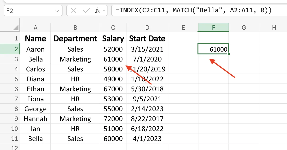
An employee table where the name Bella appears in both the Marketing and Sales departments

There are two ways to do it. Start with the easy one.

The Easy Way: A Helper Column

Add a column that glues the name and department together. In a spare column, say E2, type:

=A2&B2

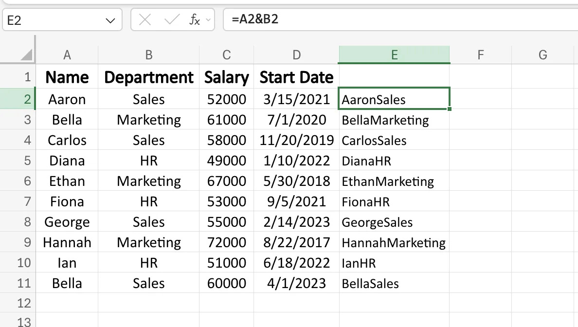
A helper column joining each employee's name and department into a single value

Copy it down. Now row 3 reads "BellaMarketing" and row 11 reads "BellaSales". Each one is unique, so you can look it up like any normal value:

=INDEX(C2:C11, MATCH("BellaSales", E2:E11, 0))

It returns 60000, the Sales Bella. You turned two conditions into one, then ran a basic lookup on it. Simple, and easy to read later.

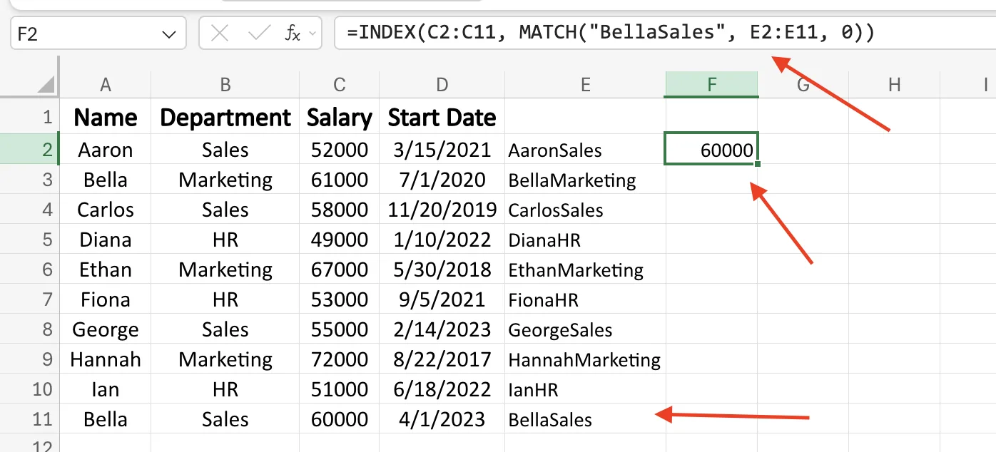
INDEX MATCH returning the salary for the Sales Bella using the helper column

The Direct Way: One Formula, No Extra Column

If you'd rather not add a column, check both conditions inside the formula itself:

=INDEX(C2:C11, MATCH(1, (A2:A11="Bella")*(B2:B11="Sales"), 0))

It returns 60000 too. The middle part looks odd, so here's what it does.

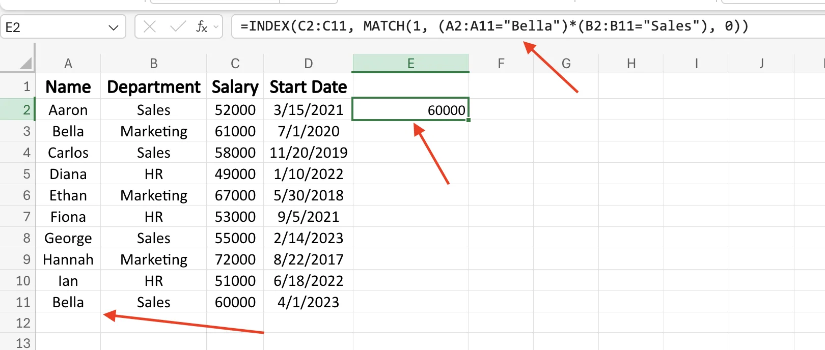
A single INDEX MATCH array formula that matches on both name and department

(A2:A11="Bella") checks every name and marks each row TRUE or FALSE. (B2:B11="Sales") does the same for departments. Multiply them, and Excel reads TRUE as 1 and FALSE as 0. A row comes out as 1 only when both are true. Every other row becomes 0.

So you get a column of 0s with a single 1, on the Sales Bella's row. MATCH(1, ...) finds that 1, and INDEX returns the salary next to it.

Need more conditions? Keep multiplying: (...)*(...)*(...). Each one is another "and this must also be true."

One catch: in older Excel versions, finish this formula with Ctrl+Shift+Enter instead of Enter. In Excel 365 and Google Sheets, plain Enter works.

INDEX MATCH vs VLOOKUP and XLOOKUP

INDEX MATCH isn't Excel's only lookup option. VLOOKUP came first, and XLOOKUP is the newest. Here's how they compare.

Feature	VLOOKUP	INDEX MATCH	XLOOKUP
Looks left	No	Yes	Yes
Survives moved columns	No	Yes	Yes
Works in old Excel	Yes	Yes	No
Easy to write	Yes	Medium	Yes
Fast on big sheets	No	Yes	Yes

VLOOKUP is the easiest to learn, but it's also the most limited. It can only look to the right, and formulas can break if columns are inserted or moved.

XLOOKUP solves both of those problems. It can look in any direction, has a simpler syntax, and includes built-in error handling.

INDEX MATCH takes a little more effort to learn, but it's flexible, reliable, and works in every modern version of Excel, including older versions where XLOOKUP isn't available and returns a #NAME? error. That's why many teams that share workbooks across different Office versions still rely on it.

One thing that makes INDEX MATCH easier to remember is that it uses almost the same pieces as XLOOKUP, just arranged differently.

XLOOKUP

=XLOOKUP(lookup_value, lookup_array, return_array)

INDEX MATCH

=INDEX(return_array, MATCH(lookup_value, lookup_array, 0))

Another useful tip is to wrap the formula in IFNA so users see a friendly message instead of #N/A when no match is found:

=IFNA(INDEX(C2:C11, MATCH(F2, A2:A11, 0)), "Not found")

This way, Excel displays "Not found" instead of an error whenever the lookup value isn't in the list.

Common INDEX MATCH Errors and How to Fix Them

INDEX MATCH is reliable, but a few small mistakes trip up almost everyone. Here are the most common ones and the quick fix for each:

Missing the 0 in MATCH. Without the final 0, MATCH doesn't perform an exact match and can return the wrong row on unsorted data. Always end MATCH with 0:

=INDEX(C2:C11, MATCH(F2, A2:A11, 0))

Ranges shift when you copy the formula. If you copy the formula down, the lookup ranges move unless you lock them. Use $ to keep the ranges fixed while the lookup cell changes:

=INDEX($C$2:$C$11, MATCH(F2, $A$2:$A$11, 0))

The ranges don't line up. The range that INDEX returns from and the range that MATCH searches must cover the same rows. If one is A2:A11 and the other is C2:C10, the positions won't line up and the formula can return incorrect results. Make sure both ranges have the same start and end rows.
A value that's clearly there won't match. The most common cause is an extra space. For example, "Aaron " (with a trailing space) won't match "Aaron". Remove extra spaces with TRIM, or correct the original data.
You get #N/A. This means MATCH couldn't find the lookup value. Either the value isn't in the list, or there's a data type mismatch: for example, the number 100 stored as text ("100"). Check that the value exists and that both sides use the same data type.

Skip the Formula: Let GPT for Work Handle INDEX MATCH for You

INDEX MATCH works well when your data is clean. It expects exact matches, so it finds "Bella" only if the cell contains "Bella", letter for letter. It won't know that "Bob" and "Robert" refer to the same person, or that "NYC" and "New York" mean the same place. Real spreadsheets are rarely that tidy, and that's where formulas start to struggle.

GPT for Work takes a different approach. It's an AI agent that works directly inside Excel and Google Sheets. Instead of building formulas, you describe what you want in plain English, and it reads your data and returns the results.

For example, you could ask:

"Pull the salary and department for Carlos and Hannah. Bella appears twice, so use the one in the Sales department. Then calculate how many years each of the three has worked here based on their start date."

That request involves multiple lookups, selecting the correct Bella from two matches, and calculating years of service from a date. With traditional Excel formulas, you'd likely need a multiple-criteria INDEX MATCH, additional formulas, and perhaps a helper column. GPT for Work handles the entire request in one step.

And it isn't limited to lookups. The same AI agent can clean messy dates, categorize thousands of rows, rewrite text, summarize data, translate entire worksheets, and much more, all from a simple prompt.

Installation takes about 30 seconds, and you can get started for free.

Conclusion

INDEX MATCH comes down to two simple jobs: MATCH finds the position of a value, and INDEX returns the value at that position. Together, they let you look up almost anything in a worksheet, from a single salary to the value where a row and column intersect. Unlike VLOOKUP, the formula keeps working even if columns are moved or inserted.

Start with the basic lookup until it feels natural. Then build on it with two-way and multiple-criteria lookups as your spreadsheets become more complex. Remember to use 0 in MATCH for exact matches and lock your lookup ranges with $ when copying formulas to avoid the most common mistakes.

And when the task becomes too large or too complex for a single formula, GPT for Work can take over. Instead of building nested formulas, just describe what you want in plain English, and the AI handles the work across your entire spreadsheet in both Excel and Google Sheets.

FAQs

What's the difference between INDEX and MATCH?

They do opposite jobs. MATCH takes a value and tells you its position in a list. INDEX takes a position and gives you the value sitting there. You combine them so MATCH finds the row and INDEX returns the answer from it.

Why use index match instead of VLOOKUP?

Index match looks in any direction, including to the left, which VLOOKUP can't. It also doesn't break when you add or move columns, and it's faster on large sheets. VLOOKUP is simpler to write, but it's more fragile.

Is index match still worth learning if I have XLOOKUP?

Yes. XLOOKUP is easier on modern Excel, but it doesn't exist in older versions, so files built with it show errors when shared with someone on Office 2016 or earlier. Index match runs on every version, which is why many teams still rely on it.

Can index match return more than one match?

No. It returns the first match and stops. If you need every matching row, use the FILTER function instead, which pulls all of them.

Why does my index match return #N/A?

MATCH couldn't find the value. Either it isn't in the list, there's a hidden space (like "Aaron " instead of "Aaron"), or it's a number stored as text. Check the value exists and that both sides are the same type.

Does index match work in Google Sheets?

Yes, exactly the same way. The same formulas you write in Excel work in Google Sheets with no changes.