So you opened a spreadsheet, and Excel suddenly showed you a warning about a "circular reference." Maybe some of your numbers turned into zeros. Maybe something just doesn't add up.
If you have no clue what happened, don't worry. You're in the right place.
A circular reference sounds complicated, but it's actually simple. It means one of your formulas is pointing back to itself, either directly or through other cells, so Excel gets stuck in a loop.
This can happen easily, especially when you're working in a spreadsheet someone else created.
The tricky part is figuring out exactly which formula is causing the problem.
That's what we'll fix here. If you want to know how to find circular references in Excel, you'll see exactly where to look and how to fix them, even if you've never dealt with one before.
Most of the time it's a quick fix once you know the steps. But first, let's look at what a circular reference actually is.
What Is a Circular Reference in Excel?
A circular reference happens when a formula depends on its own result. Excel tries to calculate it, but the answer keeps pointing back to itself, creating a loop.
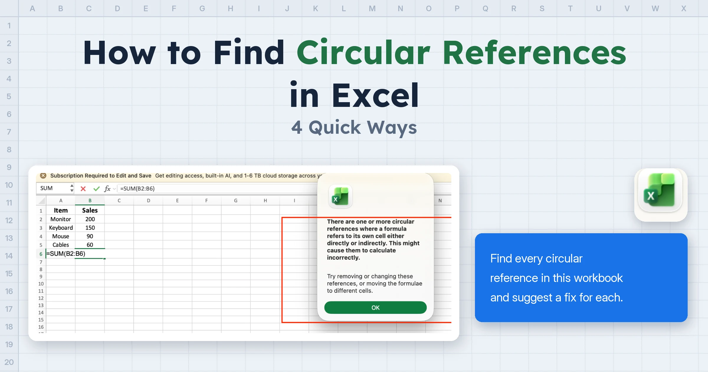
Here's the simplest way to picture it. Say you have a few sales numbers:
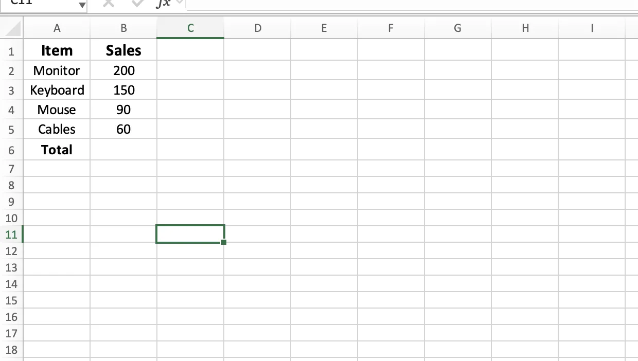
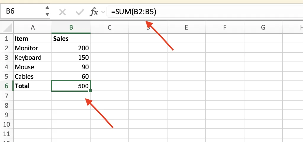
You want a total in cell B6, so you type =SUM(B2:B6). But look closely. You just told B6 to add up everything from B2 to B6, and that range includes B6 itself.
Excel can't calculate B6 without using the value of B6 itself. So it shows you a circular reference warning.
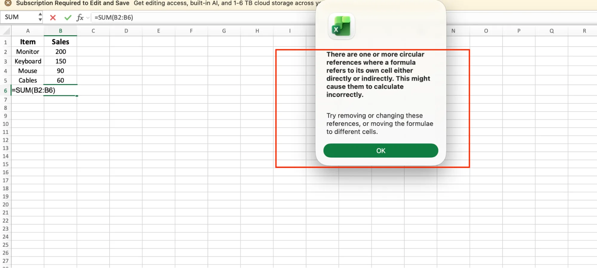
There are two types, and it helps to know the difference.
The first is a direct circular reference. That's the example above, where a cell refers to itself in its own formula. These are usually easy to catch.
The second is indirect. This is when cell A refers to cell B, and cell B eventually refers back to cell A. Each formula may look fine on its own, so these are much harder to spot.
Either way, a circular reference can prevent Excel from calculating the affected formulas correctly. That's why your numbers may suddenly look off.
Not every circular reference is a mistake, though. Some advanced spreadsheets use them on purpose, with iterative calculation enabled, and we'll cover that later.
Method 1: Check the Status Bar (Fastest Way)
The fastest way to find a circular reference in Excel is to look at the bottom of your window. Excel can show the circular reference right there on the status bar, and most people never notice it.
When the warning pops up, click OK to close it first. You can then use the status bar to locate the circular reference.
Now look at the bottom-left of the screen. You'll see text like "Circular References: B6." That's Excel pointing you straight to a cell involved in the problem.
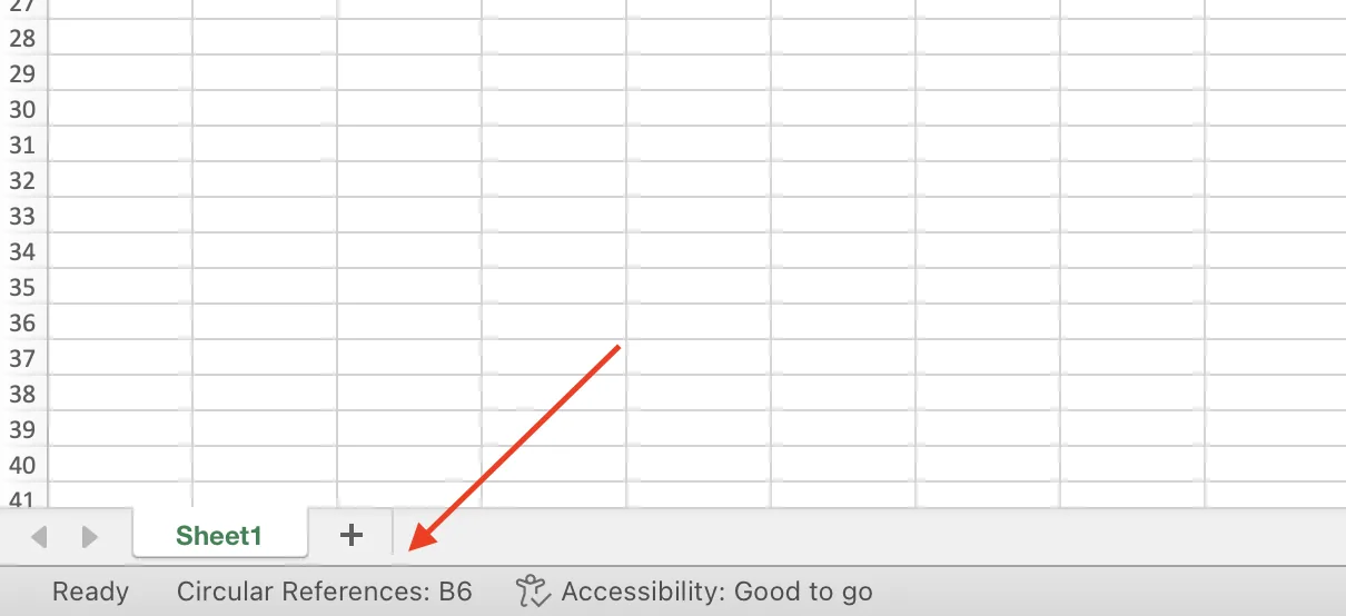
To jump right to that cell, press Ctrl + G, type the cell address (like B6), and press Enter. Excel takes you straight there.
There's one catch. The status bar may only show one circular reference, even if your file has more than one. After you fix the first, check the status bar again to see if another address appears.
Method 2: Use Error Checking in the Formulas Tab
The status bar is quick, but if you want another way to locate the problem, use Excel's Error Checking tool. You can access it at any time, even after you've closed the warning.
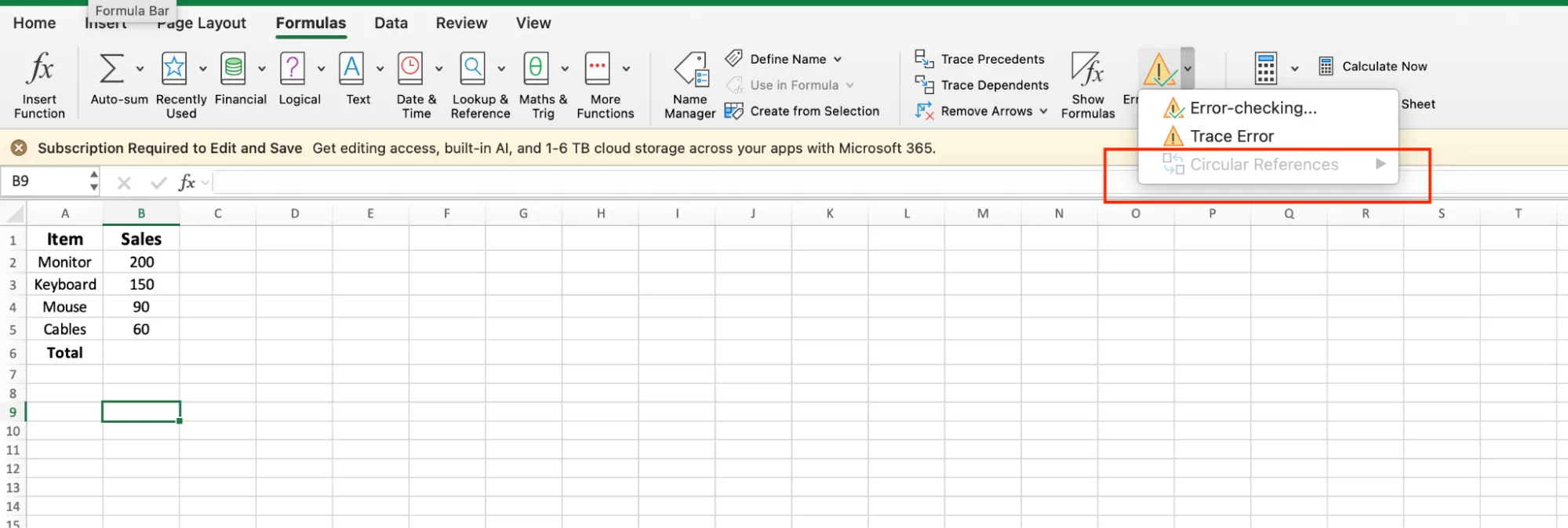
Go to the Formulas tab on the ribbon. In the Formula Auditing group, click the small arrow next to Error Checking.
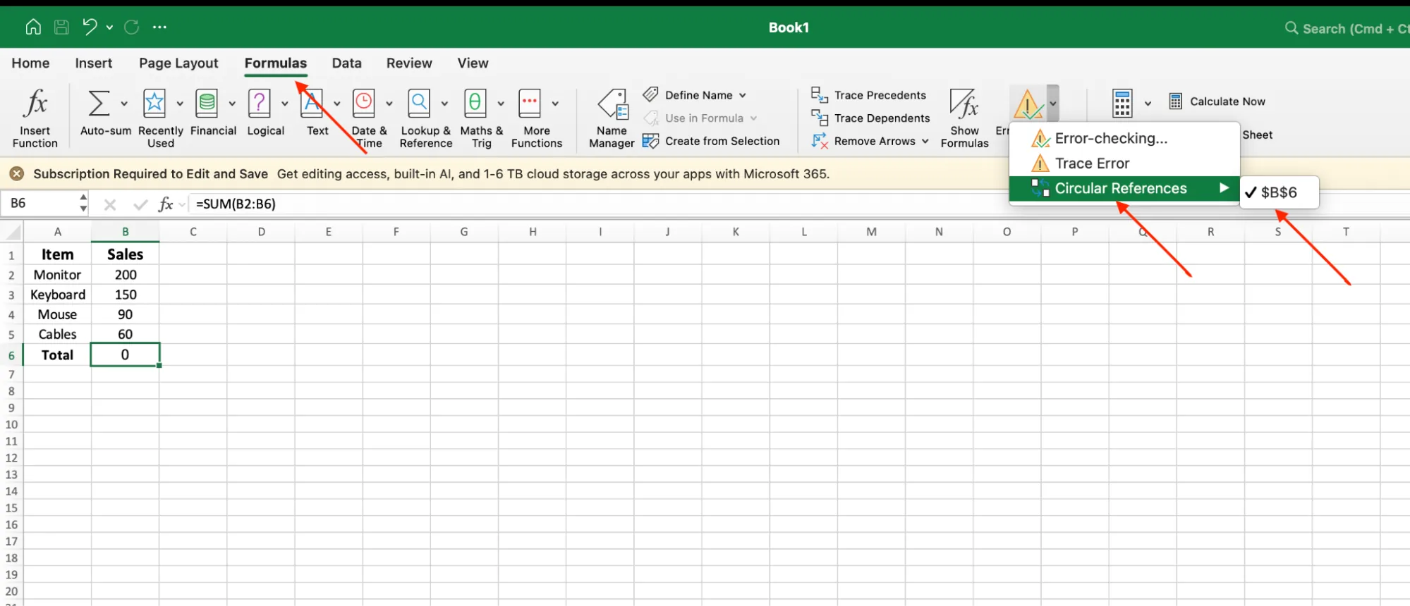
Hover over Circular References in the menu. Excel shows the address of a cell involved in the circular reference, like B6. Click it, and Excel jumps straight to that cell.
Like the status bar, Error Checking may not show every cell involved in the loop at once. Fix the listed reference, then open the menu again to check whether any circular references remain.
Here's how you know you're done. When Circular References is greyed out and no cell addresses appear in its submenu, Excel isn't detecting any remaining circular references in the workbook.
For larger workbooks, repeat the process after each fix. A circular reference can involve formulas across different worksheets, so you may need to trace cells on more than one sheet.
Method 3: Trace the Problem With Precedents and Dependents
Sometimes Excel points you to a cell, but that's not where the real problem started. One cell depends on another, which depends on another, and somewhere in that chain, a cell refers back to the start.
When that happens, you need to see how the cells connect. Excel has two tools for this, and they draw arrows between related cells so you can follow along.
They're called Trace Precedents and Trace Dependents, both on the Formulas tab.
Let's use a quick example. Say you have this small budget sheet:
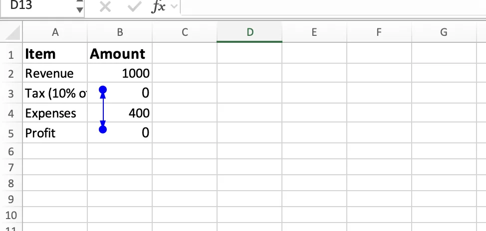
Trace Precedents shows which cells provide values to the cell you picked. Trace Dependents shows the other way around: which cells depend on the selected cell. Use both, and you can follow the chain step by step.
Here's how:
- Click the cell Excel flagged (from Method 1 or 2). In our example, that's B5.
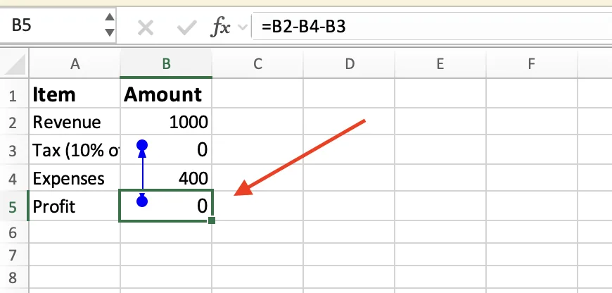
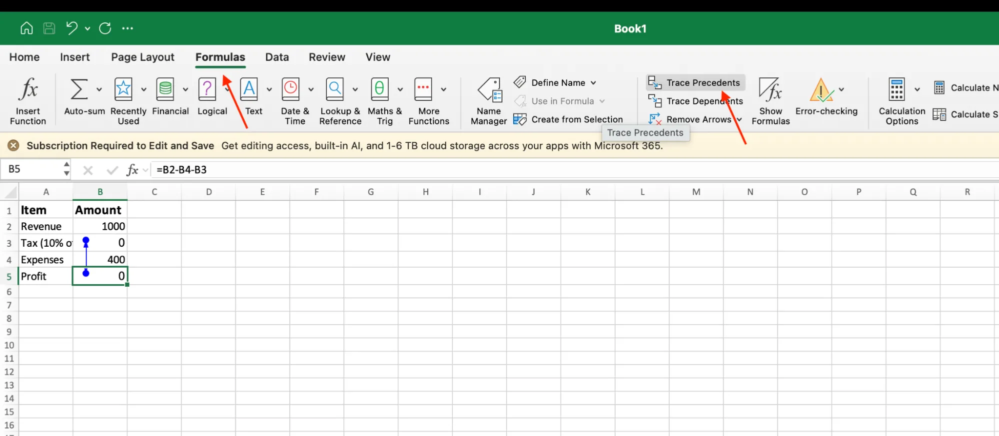
- On the Formulas tab, click Trace Precedents. Blue arrows appear, pointing to B2, B4, and B3.
-
Follow the arrows to see how the cells are connected.
-
Click B3, then click Trace Precedents again. An arrow points right back to B5.
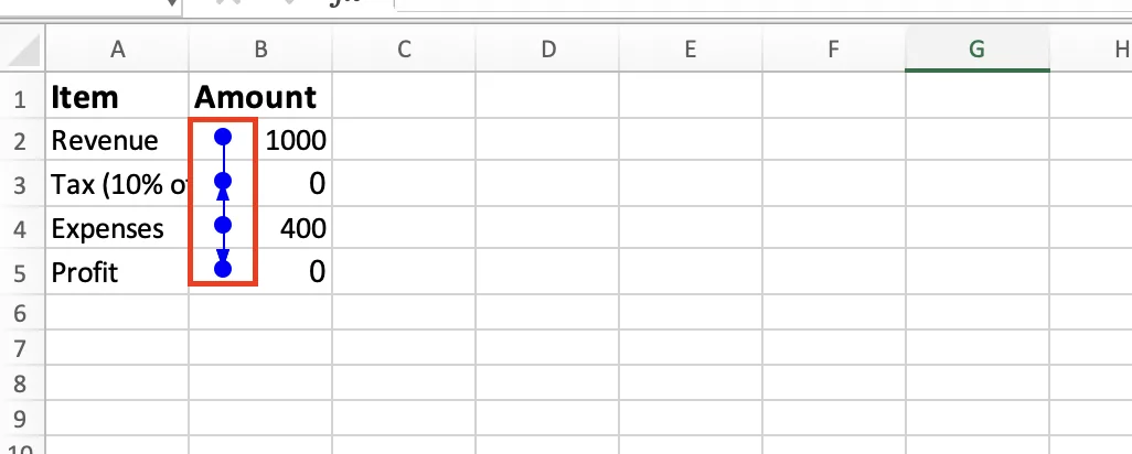
- There's your loop. B5 needs B3, and B3 needs B5. When you're done, click Remove Arrows to clean it up.
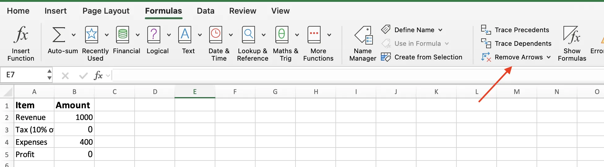
This is the surest way by hand to catch a loop that hides on another sheet or inside a named range. The arrows show you the full picture when the menus can't.
Method 4: Find and Fix Circular References Automatically With GPT for Excel
The first three methods work, but they all share the same problem. They're manual, and troubleshooting can take time when a file has dozens of tabs or complex formulas.
What if you could just ask an AI agent in your spreadsheet to find the problem for you?
Not just get a tip on where to look. Have it trace the circular reference, explain what's causing it, and suggest how to fix it.
That's what GPT for Excel does. It's an AI agent that works right inside Excel. You tell it what you want in plain English, and it does the work.
Open the GPT for Excel panel and type something like:
"Find every circular reference in this workbook, tell me which cells cause each one, and suggest a fix for each."
It reads the whole workbook, follows the chain across every sheet, and tells you exactly which cells form each loop and why. It can suggest the corrected formula too, so you're not left guessing.
That's the difference. The manual methods point at one cell and stop. GPT for Excel checks everything, explains the cause, and gives you the fix.
And circular references are just the start. Almost anything you'd normally do by hand in Excel, you can ask GPT for Excel to do for you in a single prompt.
How to Fix a Circular Reference Once You Find It
Finding the cell is half the job. Now let's fix it. There are three common ways, and which one you use depends on what caused the loop.
1. Adjust the range
This is the most common cause. It happens when a formula's range accidentally includes the cell the formula sits in, usually when a SUM or other total extends one row too far.
The fix is to shorten the range so it stops just above the formula cell.
For example, in our sales table B6 had =SUM(B2:B6), which included B6 itself. Changing it to =SUM(B2:B5) stops the range right above the total, and the loop is gone.
2. Re-point the reference
Use this when two cells depend on each other. One cell needs a value from a second cell, and that second cell is calculated from the first.
Break the loop by pointing one of the formulas at a different cell or value instead.
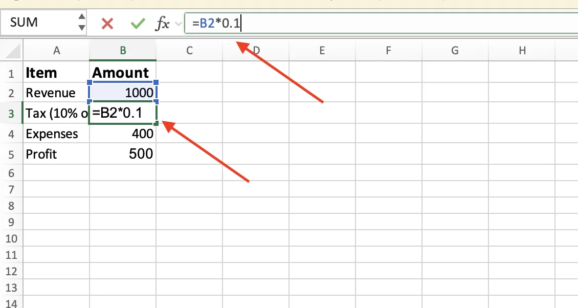
In our budget example, Profit (B5) needed Tax (B3), and Tax was worked out from Profit. Basing the Tax on Revenue instead, so B3 becomes =B2*0.1, breaks the loop because nothing points back anymore.
3. Rebuild the logic
Sometimes one fix isn't enough because the whole setup loops. The final result feeds back into its own calculation through several steps in between.
When that happens, rethink how the formulas depend on each other. You may need to move the final result out of the calculation chain or change which cells are used as inputs.
The rule to remember is short. A cell can never be part of its own calculation, directly or through other cells. Keep the result out of the chain and the circular reference stays gone.
When a Circular Reference Is on Purpose (Iterative Calculation)
Not every circular reference is a mistake. Some advanced spreadsheets actually use them intentionally.
The classic case is finance. Think of a financial model where one calculation depends on another, which in turn depends on the first. That's a loop on purpose, and the model may rely on it to reach a result.
For these cases, Excel has a setting called iterative calculation. It tells Excel to recalculate the formulas repeatedly until the result converges or the maximum number of iterations is reached.
Here's how to turn it on in Windows:
- Click File, then Options.
- Go to the Formulas tab.
- Check the box for Enable iterative calculation.
- Set Maximum Iterations (how many times it loops) and Maximum Change (how precise the result is).
- Click OK.
On a Mac, the steps are nearly the same. Open Excel, click Preferences, then Calculation, and check Use iterative calculation there.
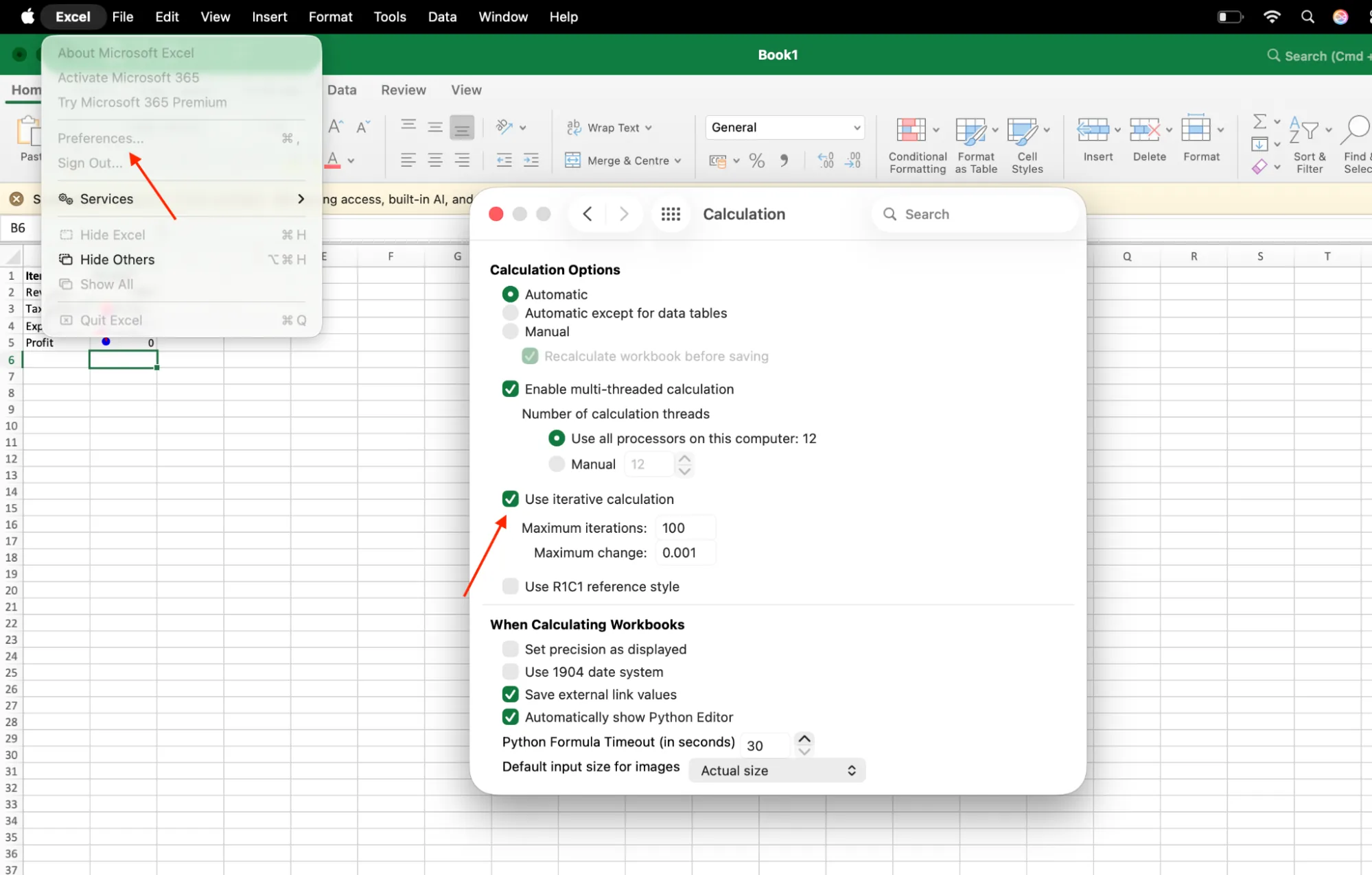
Now for the important part. Only turn this on if your model truly needs it.
If you enable it just to make a warning go away, Excel may keep calculating a circular formula instead of alerting you to the underlying problem. That can produce unexpected or inaccurate results.
So if you turned it on just to test something, turn it back off the same way. Leave it off unless a specific model depends on it.
Why Circular References Happen in the First Place
Most circular references come down to a few simple mistakes. Once you know the causes, they're easy to avoid.
Here are the usual causes:
-
The range goes one cell too far. You write a
SUMfor a total, but the range includes the total cell itself. This is one of the most common causes. -
You copied a formula. You drag a formula across or down, and somewhere along the way it ends up pointing back at its own cell.
-
Two summary cells reference each other. One total pulls from another total, and that one eventually points back to the first. This is common in budgets and financial models.
-
A named range or another sheet loops back. The circular reference isn't obvious because the loop hides behind a named range or sits on a different worksheet.
The easiest way to avoid the most common circular reference is one quick habit. Before you confirm a total, check that the selected range stops one row above the formula cell.
Conclusion
A circular reference looks scary at first, but it's usually a quick fix once you know where to look.
Start with the status bar. It can point you to a cell involved in the circular reference right away. If you need another way to find it, use Error Checking on the Formulas tab. For tricky loops that involve multiple cells or sheets, follow the trace arrows. And when a file is too big to check by hand, you can install GPT for Excel and have it find and troubleshoot circular references from a prompt.
Whichever method you use, the main rule is the same. A cell can't be part of its own calculation. Keep the answer out of the loop, and the warning stays away.
Next time that warning pops up, you'll know just what to do.
FAQs
Why does Excel say "there are one or more circular references" when I open a file?
It means a formula somewhere in the file points back to its own cell, directly or through other cells. The file still opens, but the looped cells usually show zero. Use Method 1 or 2 above to find which cell it is.
How do I find a circular reference Excel won't show me?
Sometimes the status bar stays blank or the loop sits on another sheet. When that happens, check each sheet one by one with Error Checking, then use Trace Precedents to follow the path. Loops hidden inside named ranges almost always need the trace arrows.
What does a circular reference error actually do to my numbers?
Excel can't finish the math, so it usually returns zero for the looped cells and any cell that depends on them. Your totals look wrong until you fix the loop.
Can I just leave a circular reference in my file?
Only if it's intentional and you've turned on iterative calculation for it. Otherwise no, because Excel will show wrong numbers instead of warning you.
Is a circular reference the same as a circular formula?
Yes. Both mean the same thing, a formula whose result depends on itself.